opthash: From Paper to Hardware and Back
From Paper to Code
Earlier this year, a Quanta video about recent breakthroughs in computer science covered a theoretical result that stuck with me: a new way to build open-addressed hash tables. In open addressing, every key and value lives directly in one array. When a key hashes to a slot that is already taken, the table walks a fixed sequence of other slots, called the probe sequence, until it finds an empty one. That walk is why tables slow down as they fill: the fuller the array, the more occupied slots a key steps past before it finds room.
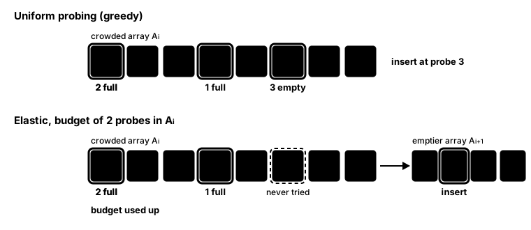
The paper behind the result, Optimal Bounds for Open Addressing Without Reordering, gives two constructions, Elastic Hashing and Funnel Hashing. Both keep insertions and successful lookups cheap even when the table is almost full, and neither ever moves an entry once placed. Elastic Hashing is the less conventional of the two. Classic schemes are greedy: they take the first empty slot their probe sequence reaches, and the paper proves a lower bound that applies to every greedy scheme. Elastic is not greedy, so that bound does not apply to it. It gives each array a probe budget, and once the budget runs out, it stops looking in that array and moves on to the next one, even if the array still has empty slots.1
I couldn’t find an official implementation, so I wrote one. Building the algorithms seemed a better way to understand them than rereading the proofs, and Rust offered control over memory layout and SIMD, plus an excuse to learn more of the language.
That became opthash. It started as an exploratory exercise. I was curious how these constructions would stack up against the tables most Rust code already relies on, like std::HashMap and hashbrown, once caches, vector instructions, allocators, and the demands of a real library got involved. As I optimized them, a harder question came up: would the faster versions still be the algorithms from the paper?
Answering that question starts with what the paper fixes. Each construction decides which arrays a key may use and the order in which it tries their slots. How a slot is checked is left to the implementation.
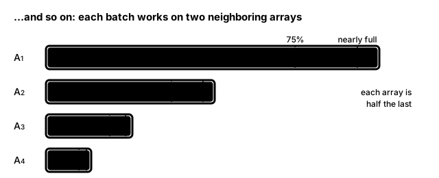
The two constructions make those choices differently. Elastic splits the table into a series of arrays, each half the size of the one before, and starts by filling the largest to about 75 percent. After that, insertions proceed in batches, each working on a pair of neighboring arrays, a larger and a smaller . A batch tops up until only a small fraction of its slots are free and fills to 75 percent, setting up the next pair.
Within a batch, two checks pick one of three cases for each key:
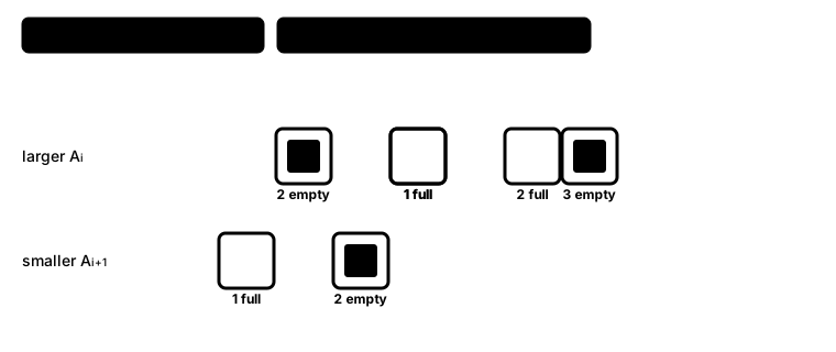
Lookups work differently: they don’t use batches or cases. A lookup can’t tell which batch placed a key, so it may have to check every array. It walks one global probe sequence that visits the arrays in a fixed, interleaved order until it finds the key.
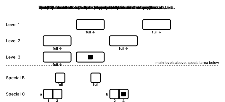
Funnel also splits the table into levels that shrink, but each main level is divided into buckets of one fixed width. A later level is smaller because it has fewer buckets, while each bucket keeps the same width. The paper derives the bucket width, level count, and shrink rate from the table’s headroom.2 An insertion falls through the levels until it finds room, and a small special area at the bottom catches what the last level can’t hold:
My first version translated these rules as literally as I could. It was easy to check against the paper, but it was slow.
Making It Fast
Version 1 mapped the paper’s structures straight onto Rust structs, with each region owning a Vec<Option<Entry>>. The code mirrored the paper’s diagrams, but every region was its own allocation, every probe chased a pointer to reach it, and every slot the probe rejected had already pulled a full entry into cache just to read its tag.
Version 1’s problems set the pattern for the rest of the project. What mattered was not how many probes an operation made, which is what the paper counts, but what each probe cost the processor. That cost depended on which cache lines the probe pulled in, which branches it mispredicted, and whether it had to load a whole key just to learn the slot was wrong.
The paper studies fixed-size, insertion-only tables, and a library needs more features than that. Those features couldn’t be measured fairly while the basic tables were still slow for hardware reasons like cache misses and pointer chasing, so I worked on performance first.
SwissTable, the design behind Abseil’s hash tables and hashbrown, was a natural model for making each probe cheaper. It stores a small hash fingerprint in each control byte and compares a whole group of them in one vector instruction, so one probe can rule out many slots.
Version 2 took the first step toward that design. It kept the regions separate but moved control metadata out of the entries and into its own array, so a lookup could check a one-byte control value before loading any key or value, and most empty or non-matching slots never touched the payload. Version 3 put every region into one allocation, keeping the logical boundaries between levels while placing all their control bytes side by side in memory.3
block-beta
  columns 10
  t1["Version 1: one Vec per level: the Option tag sits inside every slot"]:10
  a0t["tag"] a0e["L0 entry"] a0t2["tag"] a0e2["entry ..."] space a1t["tag"] a1e["L1 ..."] space a2t["tag"] a2e["L2 ..."]
  t2["Version 2: one table per level: control bytes split out"]:10
  b0["L0 slots"]:3 b0c["L0 ctrl"]:1 space b1["L1 slots"]:1 b1c["ctrl"]:1 space b2["L2 slots"]:1 b2c["ctrl"]:1
  t3["Version 3: one arena: all control bytes first, then all slots"]:10
  c0["ctrl L0 L1 L2"]:2 c1["L0 slots"]:3 c2["L1"]:2 c3["L2"]:1 c4["membership filter"]:2
  classDef ctrl fill:#f4c95d,stroke:#8a6d1d,color:#000
  classDef title fill:none,stroke:none
  class a0t,a0t2,a1t,a2t,b0c,b1c,b2c,c0 ctrl
  class t1,t2,t3 title
From there, opthash adopted SwissTable’s seven-bit fingerprints and SIMD control-byte scans, and switched to the foldhash hasher. Rounding sizes to powers of two turned some divisions into bit masks, and the single arena kept the hot control regions together and cut allocation traffic.
All of this made the maps faster and harder to measure. A layout change can shift a field or loop across a cache-line boundary, so a faster run alone doesn’t tell you which change helped, or whether the gain will hold on another machine.
The lesson that stuck came from a mini-hash experiment that never merged.4 It stored 4 extra bytes of hash per slot so a lookup could reject more candidates before comparing keys. The first run showed three Funnel workloads in the Python bindings improving by 33 to 39 percent. It looked like a clear win until I noticed the two runs had landed on different classes of CPU core, one clocked a gigahertz faster than the other. Pinned to the same core, most of the win disappeared:
| Funnel workload (Python) | First run | Pinned to one core |
|---|---|---|
| insert | 33% faster | 21% faster |
| union | 37% faster | 12% slower |
| runion | 39% faster | flat |
| lookup hit | – | 4% slower |
| median across the suite | – | flat |
A flat median wasn’t worth 4 extra bytes per slot, so I dropped the idea. More importantly, I stopped trusting wall-clock numbers on their own. The local harness now:
- pins each run to one core and fixes memory placement
- saves named baselines to compare against
- reruns the unchanged
stdandhashbrownmaps as controls for the noise floor - checks assembly and hardware counters to tell fewer instructions apart from better cache or branch behavior
Smaller experiments went through the same checks.5 Much later, I found the benchmark fixture itself was skewed: at 20,000 entries, Elastic and hashbrown were 70 percent full while Funnel was completely full. Now every map is filled to capacity before anything is measured.6
Better measurement caught wins that were noise and wins that only held on one machine. It also exposed a bigger problem. Some optimizations that measured well, notably power-of-two geometry and changed probing arithmetic, had changed which slots the algorithms visited.
The maps were faster because they were no longer quite the paper’s algorithms.
Returning to the Paper
Lining the code up against the paper showed the drift. It wasn’t one bug: several optimizations had each nudged the probe sequence, and Funnel’s bucket and overflow handling had mismatches of its own. Patching them one at a time wouldn’t yield a trustworthy reference, because another optimization might still be changing geometry or probe order somewhere I hadn’t looked.
So I rewrote both maps to follow one fixed instantiation of the paper’s constructions exactly, by default.7 Every optimization faced one test: does it change which slots get probed, or only how each slot is checked?
| Removed: changed which slots get probed | Kept: changes only how slots are checked |
|---|---|
| Power-of-two level sizes8 | Single arena |
| Triangular Elastic probing | Control bytes with fingerprints |
| Altered probe budgets | SIMD control-byte scans |
| Performance-oriented reserve policy |
To enforce that test, I wrote scalar reference implementations. Each one applies the paper’s rules in the paper’s order, without SIMD or cached state, so it is slow but easy to check line by line against the paper. Here is the reference’s Elastic insertion rule for one batch, lightly trimmed, with the same three cases as the diagram above:
// Batch i works across levels `current` (A_i) and `next` (A_{i+1}).
let free_current = self.levels[current] - self.occupancy[current];
let free_next = self.levels[next] - self.occupancy[next];
let current_threshold = floor_div_pow2(self.levels[current], reserve + 1); // δ|A_i|/2

if free_current <= current_threshold {
    // Case 2: A_i has reached its fill target. First free slot in A_{i+1}.
    self.uniform_vacancy(next, key)
} else if free_next <= self.levels[next] / 4 {
    // Case 3: A_{i+1} is already 3/4 full. First free slot in A_i.
    self.uniform_vacancy(current, key)
} else {
    // Case 1: a bounded budget of probes in A_i, computed from how
    // full it is, then fall through to the first free slot in A_{i+1}.
    let budget = probe::elastic_dyadic_probe_budget(free_current, self.levels[current], reserve, C)
        .expect("valid budget inputs");
    (0..budget)
        .find_map(|j| self.vacancy(current, key, j))
        .unwrap_or_else(|| self.uniform_vacancy(next, key))
}
The snippet is short, but three details in it explain why we pruned those optimizations specifically:
- Placement is deterministic. Each branch depends only on two occupancy counts and the key itself, so the same inserts always produce the same placements. That is what lets the reference serve as a test.
- Probes map to slots through exact sizes.
vacancy(level, key, j)checks the -th slot in the key’s probe sequence for a level, anduniform_vacancytries until one is free. The slot for each is computed from the level’s true size, so rounding sizes to a power of two sends keys to different slots. - Thresholds use integer rounding. opthash keeps a power of two, so is a bit shift (
floor_div_pow2). An optimized table has to round the same way, or a key near a threshold takes a different case.
Because the reference decides where every probe lands, it doubles as a test oracle. Tests insert the same keys into both tables and check that every key lands in the same slot at the same probe position.
flowchart LR
  in["same keys"] --> ref["Scalar reference"]
  in --> opt["Optimized table<br/>SIMD, cached state"]
  ref --> eq{"same slot and<br/>probe position?"}
  opt --> eq
  eq -- yes --> ok["same algorithm, maybe faster"]
  eq -- no --> bad["test fails: algorithm changed"]
The rewrite made both maps much slower. Here is the cost on a 20,000-entry map of u64 keys, in nanoseconds per operation, before (v0.10.3) and after the rewrite:9
| Map | Insert | Hit | Miss |
|---|---|---|---|
| Elastic | 9.4 → 110 (11.7x) | 3.7 → 32 (8.6x) | 3.7 → 264 (70x) |
| Funnel | 8.0 → 17 (2.1x) | 5.0 → 15 (3.0x) | 8.0 → 55 (6.9x) |
hashbrown | 3.6 | 2.1 | 1.9 |
These numbers compare two versions of opthash, so they show how much slower exactness made this implementation. They don’t test the paper’s bounds, which count probes rather than nanoseconds.10
I kept the slower, exact version anyway. A fast implementation of a different candidate order couldn’t answer the question that started the project: how do the paper’s algorithms behave on real hardware? From then on, the reference decided which optimizations were allowed.
Keeping it meant understanding where the time went, so I read the CPU’s hardware counters with perf. Each version ran successful Elastic lookups for five seconds on the same pinned core, old version first:
$ perf stat -e cycles,instructions,cache-misses,branch-misses speedup --profile-time 5 '^get_hit/get_hit_elastic$'

v0.10.3
    20,136,315,080  cycles
    95,752,902,677  instructions        # 4.76 insn per cycle
     1,338,515,144  cache-misses
        37,048,235  branch-misses

exact rewrite
    19,511,160,964  cycles
    92,545,663,178  instructions        # 4.74 insn per cycle
       175,001,595  cache-misses
        55,432,818  branch-misses
The totals look alike because both runs lasted five seconds. The exact version is slower, so it completed far fewer lookups in that window, and the counters only make sense per lookup. Dividing the five seconds by each version’s time per lookup from the table above gives the number of lookups each one completed:
Dividing each counter by those counts gives the cost of a single lookup. These are estimates, since the benchmark loop adds a little work of its own, but the differences are far larger than that overhead:
| Per lookup | v0.10.3 | Exact | Ratio |
|---|---|---|---|
| Cycles | ~15 | ~125 | 8.4x |
| Instructions | ~71 | ~590 | 8.4x |
| Instructions per cycle | 4.76 | 4.74 | about the same |
| Cache misses | ~1.0 | ~1.1 | about the same |
| Branch misses | ~0.03 | ~0.35 | 13x |
Cycles and instructions grew by the same factor, and instructions per cycle barely moved. The processor runs the exact version’s code just as efficiently, but there is about 8 times as much of it. Cache misses stayed near one per lookup, so on this fixture the exact hit path is not waiting on memory. The extra instructions come from following the paper: the exact version walks candidates in the paper’s interleaved order across arrays and does exact range reduction on every candidate, where the old version probed power-of-two groups using bit masks. Branch misses grew 13 times, but at about 0.35 per lookup, and roughly 10 to 20 cycles each, they account for only a few of the 110 or so extra cycles.
Insert behaves differently. There the exact version also takes about 10 times as many cache misses per operation, because it visits far more slots before it settles, and those slots are spread across two arrays instead of one contiguous group.
The first round of tuning showed the exact version had room to improve. Streamlining the hot paths made Elastic insertion about 4x faster without changing which slots it visits.11 That narrowed the project’s question to this: how fast can the paper’s design get on its own, with the library features kept out of the way?
Beyond the Paper
A real library must also delete, clear, grow, and handle a key running out of slots to try. To keep that code from changing how the paper places keys, opthash splits a table’s lifecycle into epochs. Inside an epoch, inserts and lookups follow the paper exactly. Everything else, from growth to cleanup after deletes, runs as separate library code between epochs, and each run starts a new epoch under the paper’s rules.
flowchart TB
  e1["Epoch N: paper rules"] -. "table full: grow" .-> e2["Epoch N+1: paper rules"]
  e2 -. "no allowed slot: placement recovery" .-> e3["Epoch N+2: paper rules"]
  e3 -. "cleanup, clear, or resize" .-> e4["Epoch N+3: paper rules"]
Placement recovery is the one exception. The paper gives each key a finite list of slots it may use, and under heavy churn a real table can end up with every one of them taken. When that happens, opthash does not drop the key. It first rebuilds the table at the same size, reinserting every live key into a fresh layout, which also clears out tombstones, and then tries the paper’s placement again. Only if the key still has no allowed slot does opthash put it in the first free slot it finds, a slot the paper would never have chosen for it. That placement sets a flag, so later lookups know to fall back to scanning the whole table. So “paper-exact” describes normal operation, not recovery.12
Keeping library code from changing the paper’s placements took some fixes. Elastic used to pick its active batch from a running count of inserts. Under a steady mix of inserts and deletes, that count kept climbing even though the number of live keys stayed flat, so the batch index crept forward and new keys drifted into the smallest levels, where they quickly ran out of room and set off recovery. Counting live entries instead of total inserts fixed it.13
The same split applies to benchmarks. The paper’s analysis covers inserts and successful lookups for both maps, and failed lookups for Funnel only. It doesn’t cover failed lookups for Elastic, and deletes and growth aren’t part of the paper at all, so benchmarks for those operations measure opthash’s own library code. One combined score would mix the two and hide where the time goes, so opthash reports them separately. Every run also includes std::HashMap and hashbrown, which show how fast mature, general-purpose tables are on the same machine and workload, so opthash’s numbers have something to be read against.14
Looking Back
Several lessons came from numbers that turned out to be inaccurate. The mini-hash experiment looked like a clear win until both runs were pinned to the same core, and the skewed fixture compared maps at different loads without any result looking off. Pinning the core, fixing memory placement, and rerunning an unchanged baseline like hashbrown costs a few minutes per run. It is the most reliable way I know to tell a real speedup from a lucky one.
Pinning made the numbers trustworthy, but it couldn’t tell me whether they described the right algorithm. When the goal is to study an algorithm, a speedup counts only if the algorithm stays the same. Power-of-two geometry and triangular probing are good ideas for hash tables in general. They didn’t fit here because they changed which slots get visited, and so which algorithm was measured. If I implement another paper, I will decide up front what it fixes and what it leaves open, and treat anything that moves the first as a different design.
That rule is easiest to enforce with a reference in place from the start. I wrote mine only after the optimized code had drifted, and untangling the drift took a rewrite. Built first, it would have checked every optimization the day it was written, turning “is this still the algorithm?” into a failing test instead of an audit. Speed doesn’t matter for the reference. Its only job is to be easy to check against the paper, so simple code beats fast code.
Separating the paper’s rules from the rest of the library helped too. Deletes, growth, and recovery can dominate a benchmark while saying nothing about the paper’s bounds. Separate epochs and separate benchmark groups showed which part was slow, the first step toward fixing either.
What’s Still Open
Later work kept the paper’s slot order and made each probe cheaper. A membership filter, a small Bloom filter at the end of the arena, lets most failed lookups return without probing,15 and probing itself got cheaper.16 Both maps have recovered much of the speed the rewrite cost, but neither matches hashbrown yet.
Deletes on a nearly full table are still slow. A delete-heavy workload keeps pushing Elastic into placement recovery, and each recovery rebuilds the whole table at the same size, reinserting every live key, before it can place the new one. Paying for that rebuild repeatedly is what makes these deletes slow.
opthash is licensed under Apache 2.0 and available on PyPI (pip install opthash) and crates.io (the Rust crate also builds without std).
The question that started the project is still open: can the paper’s probe bounds make opthash as fast as hashbrown in real use, without changing the algorithms again? If you would like to help answer it, the project is open source and welcomes contributions.
With uniform probing, the expected walk grows with , where is the free fraction of the array. Elastic’s budget is , where is the free fraction of the whole table. That cap is how it beats the greedy bound. ↩︎
opthash pins one such choice and treats any change to it as a different algorithm for trace purposes. ↩︎
See opthash#68. Each level became a pointer and a count into the shared arena. ↩︎
See opthash#12 for the full workload table, Elastic included. ↩︎
Software prefetching did nothing or hurt, reordering fields sometimes produced worse codegen, and a 64-lane AVX-512 path was dropped for the existing 16-lane x86 scan once the generated code showed no gain. The ARM machine used here scans 8 lanes with NEON. One change, swapping a batch-plan
Vecfor a boxed slice, lost 6.5 percent on its own and was reverted, then came back without the slowdown as part of a later layout cleanup. ↩︎See opthash#139. The fixture grew from 20,000 to 28,672 entries, the most every map can hold. ↩︎
See opthash#115. The paper leaves Elastic’s probe-budget constant free and treats its Funnel constants as sufficient rather than canonical, so “exact” here means exact to the instantiation opthash pins. ↩︎
Elastic still rounds its total size up to a power of two. The paper fixes how the space is split into arrays, not the overall table size, so this doesn’t break exactness. I tried exact total sizing anyway. It saved about 45 percent of memory at a million entries, but lookups and deletes got much slower, so I kept the power-of-two total. See opthash#137, which also lists smaller layout ideas that were tried and dropped. ↩︎
The regression was first recorded in the design notes. A fresh run for this article reproduced it: same fixtures, 100,000 operations per sample, interleaved twice on one pinned Cortex-X925 core at 3.9 GHz. At 20,000 entries, Elastic and
hashbrownare 70 percent full and Funnel is full, so compare each row before and after, not maps against each other. ↩︎Both pairs agreed within 5 percent on every cell. The
stdandhashbrowncontrols were flat on insert and hit. On miss,stdwas 1.5x slower andhashbrown0.8x in the exact tree’s binary, identically in both pairs, so that is the two bench binaries compiling the same control code differently, not run-to-run noise. ↩︎See opthash#121, which measured Elastic insert 76.63 percent faster. Its controls were noisy, so only the insert gain counts. ↩︎
The paper’s analysis assumes truly random hash functions. opthash uses fixed mixers instead, built from wyhash’s default secrets and SplitMix64’s constants. So “paper-exact” holds for opthash’s own hashing, but it isn’t a proof that fixed mixers inherit the paper’s bounds. ↩︎
See opthash#135. Over 100,000 mixed inserts and deletes, recovery rebuilds went from 11 to zero. ↩︎
The Python bindings need the same care. Python hashing, interpreter overhead, the GIL, and the PyO3 crossing can cost more than the Rust operation underneath, so those numbers measure a binding workload rather than the table. ↩︎
See opthash#132. Each key sets two bits in a 64-bit word shared by ten slots. Bits are never cleared one key at a time, so the filter can wrongly say “maybe” but never wrongly say “no”. ↩︎
See opthash#135. ↩︎