Optimizing Matrix Multiply on CUDA, Part 2
In late summer 2026, I returned to the SGEMM (single-precision matrix multiply) kernel from Part 1. Almost two years had passed since the course project, and although I no longer had access to its T4 GPU, I now had an NVIDIA GB10 to experiment with. The course kernel reached about 60% of cuBLAS’s throughput on the new GPU, leaving room to continue the optimizations we had stopped short of implementing.
The starting configuration is unchanged: a block of 256 threads computes a 128×128 tile of , with each thread keeping an 8×8 patch of running sums in registers. To update those sums, the block works through , the inputs’ shared dimension, copying slices of and from global memory into shared memory. Each thread then reads the shared copies into registers for its multiply-adds. Global memory is off-chip, while shared memory is the on-chip scratchpad of a streaming multiprocessor (SM). Part 1 improved throughput by reusing inputs across outputs; this follow-up examines the cost of moving those inputs and how much independent work the GPU has available while loads are in progress.
The course project stopped around kernel 5 of Simon Boehm’s worklog, so the later kernels provided a starting point for this solo follow-up. The T4 analysis had suggested several things to investigate: instruction overhead, a register count that allowed only one block per SM, and matrix sizes that left some SMs idle. On the GB10, these experiments eventually brought the kernel to roughly cuBLAS’s throughput, although several plausible changes did little to help.
The GB10
All timings in this post come from the GB10, the Blackwell chip in NVIDIA’s DGX Spark. I refer to the initial sequence of changes below as round two, following the course project in Part 1.
The GB10 has almost four times the T4’s peak FP32 throughput, but slightly less memory bandwidth. Its resources differ in a few other ways too:
- 48 SMs rather than 40.
- 100 KB of shared memory per SM rather than 64 KB. The register file is still 64K registers.
- About 29.5 TFLOP/s of peak FP32 compute, versus 7.68 on the T4.1 A TFLOP/s is a trillion floating-point operations per second.
- One memory shared by CPU and GPU, with 273 GB/s of bandwidth. That is about 15% less than the T4’s 320 GB/s.
To measure the remaining gap, I benchmarked both the course kernel and cuBLAS on the GB10; the T4 timings from Part 1 serve only as background. cuBLAS runs with TF32 disabled so that both implementations use full-precision FP32 inputs. Allowing cuBLAS to use lower-precision inputs would change the comparison.
The intermediate kernels are in next/, together with a small standalone benchmark. Each kernel adds a step to the previous version, and all outputs are checked against cuBLAS.2 The table summarizes this sequence at and .
| Step | vs cuBLAS | vs cuBLAS | ||
|---|---|---|---|---|
| Our course kernel | 9,661 | 60% | 10,723 | 63% |
| + two blocks per SM | 11,508 | 71% | 12,616 | 74% |
+ float4 loads, transposed | 13,882 | 86% | 14,181 | 83% |
| + bank-conflict fix | 14,323 | 88% | 14,623 | 85% |
| + warp tiling | 14,234 | 88% | 14,812 | 87% |
| + warp tiling, | 14,687 | 91% | 15,209 | 89% |
| + double buffering () | 14,933 | 92% | 15,392 | 90% |
| cuBLAS | 16,204 | 100% | 17,119 | 100% |
Allowing a second block per SM and widening the loads account for most of the improvement in this sequence. The later changes bring the kernel to about 90% of cuBLAS’s throughput, compared with roughly 60% for the course kernel.
Two Blocks per SM
The first constraint appears in the compiler’s register allocation: the course kernel uses 168 registers per thread on the GB10. Shared memory can accommodate two blocks, but the register file cannot hold two 256-thread blocks at that allocation. Adding __launch_bounds__(256, 2) to the kernel declaration asks the compiler to target two resident blocks, with no more than 256 threads in each. That leaves a budget of registers per thread:
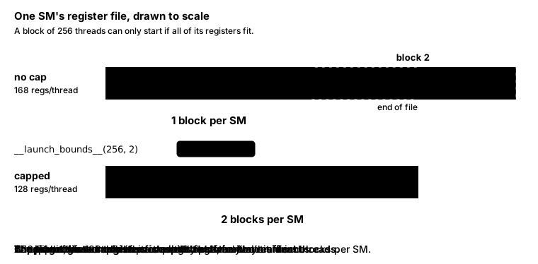
Fitting that budget requires the compiler to spill 72 bytes per thread, equivalent to 18 floats, into local memory. Despite the name, local memory is off-chip; “local” means that the storage belongs to an individual thread. The extra stores and loads could offset the benefit of a second resident block, but at the kernel still runs 19% faster. That result is consistent with the second block hiding more latency than the spills add, as anticipated in Part 1. I kept the register cap for the next experiments, accepting the spills, less register space for loading inputs early, and the 256-thread maximum block size.
Wider Loads and Bank Conflicts
Part 1’s roofline analysis suggested that the kernel already reused enough global-memory data that fetching fewer bytes per multiply-add was unlikely to improve throughput much further. The next question was how much work the SM spent moving that data. Even when the number of bytes stays the same, wider loads can reduce the instructions needed to bring the inputs into registers.
Loading Four Floats at a Time
A float4 load transfers four floats in one instruction, reducing the global-load instruction count to a quarter of the scalar version’s count. The next kernel combines these loads with a transpose of in shared memory and improves throughput by 21% at . Testing the two changes separately showed that, at this size, the gain came from the wider global loads rather than the transpose.
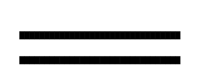
The transpose follows Boehm’s kernel and has a separate purpose. Thread 0 computes rows 0–7 and columns 0–7 of , requiring eight values from and eight from at each step through the slice. Without the transpose, its values lie in a column, 32 floats apart. Transposing the shared copy places those eight values next to one another, making it possible to read them with two wide instructions instead of eight scalar ones. The figure compares the locations of those eight inputs before and after transposing the shared copy:
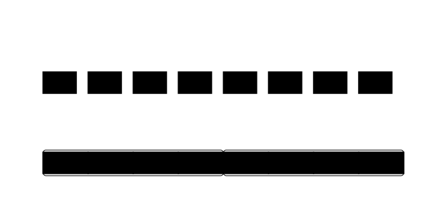
Inspecting the compiled kernels showed why this expected saving did not appear. Without the transpose, the compiler had already combined values from four successive loop steps into wide reads. Both versions issued 128 wide shared-memory reads per thread per slice, and both profiler runs recorded 16.8 million shared-memory read instructions at . The transpose therefore did not reduce the read instruction count on the GB10 in this configuration. I left it in place for the following experiments because removing it from a later kernel with a larger per-thread patch reduced throughput by 2–4%.
Changing the Shared-Memory Access Pattern
The bank conflicts suspected in Part 1 offered another place to look. Shared memory has 32 banks, with successive floats assigned to successive banks. In ’s tile, columns 0, 32, 64, … therefore map to bank 0, columns 1, 33, 65, … to bank 1, and so on. When threads request different values from the same bank, the hardware needs separate passes to serve them. Padding the array is one way to change that mapping; here, I changed which columns each thread reads.
In the previous layout, each thread handled eight consecutive columns of and read them four values at a time. Thread 0 handled columns 0–7, thread 1 handled 8–15, and thread 4 began at column 32. Because bank numbering repeats every 32 columns, the first reads from threads 0 and 4 requested different values from the same banks, creating conflicts.
Splitting each thread’s columns into two groups of four, separated by 64 columns, changes those requests. Thread 0 now reads columns 0–3 and 64–67, while thread 1 reads 4–7 and 68–71. Across eight neighboring threads, the first groups cover columns 0–31 without repeating a bank. The second groups are read by separate instructions, so they do not compete with the first groups even though their bank numbers repeat. The rows assigned from receive the same split:
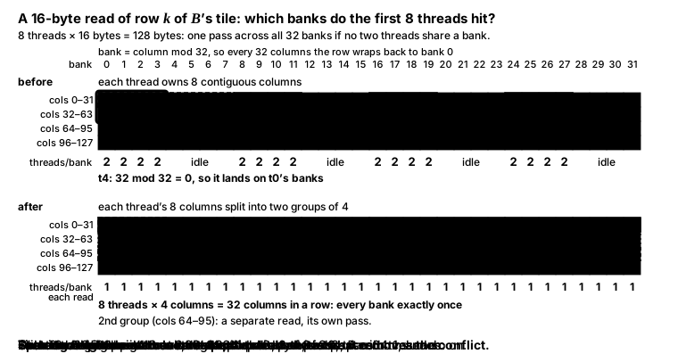
With this mapping, the profiler’s shared-memory read bank-conflict count falls from 33.6 million to 54 thousand, and throughput improves by about 3%. The average number of passes per read falls from five to three. That average includes all shared-memory reads in the kernel, so it does not imply that the reads shown above still require three passes.
Assigning a Compact Tile to Each Warp
Changing the region of assigned to each warp might reduce the shared-memory data it needs. Previously, one warp owned 16 full-width rows of the block’s tile. With warp tiling, it instead owns a compact 32×64 region, requiring 96 distinct shared-memory values per step rather than 144:
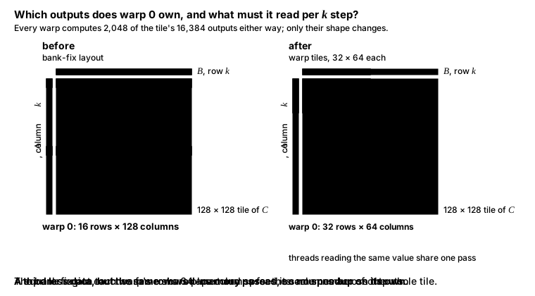
Despite the reduction in distinct values, warp tiling did not meaningfully improve runtime. In the earlier mapping, several threads requested the same value, allowing the hardware to serve those reads together. Counting distinct inputs alone therefore overstated the reduction in memory work: the profiler still recorded about 50 million shared-memory passes for either kernel. Both versions also compute the same 128×128 block tile from the same global-memory slices, so this change does not affect arithmetic intensity, the ratio of flops to bytes fetched from global memory.
Reducing the Slice Depth
The transposed layout introduces another cost when storing into shared memory. Those stores can conflict too, and reducing the slice depth from 32 to 16 halves the number of passes they require. This change adds about 3% to throughput.
For these stores, each thread writes one float, and the destination bank depends only on which row of it copied. At a depth of 32, eight threads in a warp copy values from the same row, requiring eight writes to one bank and therefore eight passes. At a depth of 16, only four threads share the row, matching the profiler’s four passes per store. The stores are still not conflict-free, but reducing the slice depth cuts that particular source of serialization in half.
Closing the Gap to cuBLAS
After reducing load instructions and bank conflicts, the kernel is within about 10% of cuBLAS’s throughput. The remaining load latency suggested a different approach: instead of only making data movement cheaper, the block could begin loading the next slice before it finished computing with the current one.
Overlapping Loads and Computation
Double buffering provides a second shared-memory buffer so that loads for the next slice can overlap computation on the current slice. In this version, the global loads first bring the next slice into registers. After computation on the current slice finishes, the threads store those prefetched values into the other shared-memory buffer, synchronize, and swap the buffers’ roles:
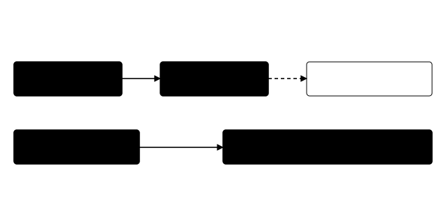
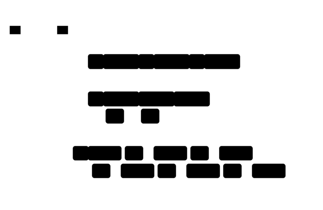
This could reduce time spent waiting at __syncthreads(), but the measured gain is only about 2%. One possible explanation is that the two resident blocks already provide much of this overlap, with one block computing while the other waits. A second buffer allows overlap within a block as well, at the cost of doubling its shared-memory use:
The GB10 supports another way to overlap data movement: cp.async, introduced with Ampere after the T4’s Turing architecture. This instruction copies directly from global to shared memory without passing through registers, and allows the kernel to queue slices across several buffers, or stages. It seemed worth testing whether that mechanism could reduce the remaining gap to cuBLAS.
In these runs, asynchronous copies did not outperform the double-buffered kernel. The table includes that result and the later increase in per-thread outputs, which eventually brought the kernel to cuBLAS’s throughput:
| Step | vs cuBLAS | vs cuBLAS | ||
|---|---|---|---|---|
| Double buffering (from round two) | 14,933 | 92% | 15,392 | 90% |
| + asynchronous copies | 14,490 | 89% | 15,384 | 90% |
| + 16×8 outputs per thread, 128×256 tile | 16,625 | 103% | 17,839 | 104% |
| cuBLAS | 16,204 | 100% | 17,119 | 100% |
I tested two configurations with the same shared-memory capacity: two stages with a slice depth of 16, and four stages with a depth of eight. The two-stage version roughly matched plain double buffering, while the four-stage version was about 5% slower. To understand why overlapping more loads had not helped, we need to distinguish the time spent waiting for data from the cost of issuing the instructions that move it.
Investigating the Cost of Copying
Removing parts of the kernel gives a rough way to investigate those costs. At , the double-buffered kernel reached about 15.7 TFLOP/s in this set of experiments. Removing its global loads raised throughput to 20.2 TFLOP/s, almost 30% higher; restoring only the shared-memory stores brought it back to 18.7 TFLOP/s. These modified kernels no longer perform a useful matrix multiplication, so their reported throughput only indicates how runtime changes when those operations are removed. Removing a load eliminates both its instruction and any wait for its result, which leaves the two possible costs unresolved.
A separate probe repeatedly copied the same slice, retaining the copy instructions while avoiding the wait on global memory. It reached the same 15.7 TFLOP/s as the real kernel, suggesting that global-memory latency was not the main cost. Stall samples supported that interpretation: 5% were associated with waiting on global memory, compared with 18% on shared memory and barriers in the double-buffered kernel. Asynchronous copies were addressing a relatively small source of waiting, and constructing the transposed tile still required one cp.async instruction per four-byte float. The change therefore did little to reduce the copy instruction count either.
Increasing the Outputs per Thread
cuBLAS’s logs suggested another direction. At , it selected a CUTLASS kernel computing 128 outputs per thread, twice the 64 in the current 8×8 patch. Giving each thread a 16×8 patch achieves the same output count in our kernel. With 256 threads and two cp.async stages retained, the block’s output tile grows to 128×256.
The larger patch lets each thread reuse its inputs across more multiply-adds. Thread 0 now loads 24 values for 128 multiply-adds per step, compared with 16 values for 64 previously. Computation doubles while loads increase by only half, reducing the shared-memory loads from four to three per 16 multiply-adds. Math-unit utilization rises from 58% to 70%.

Holding the larger patch raises the register count to 237 per thread, leaving room for only one block per SM again. This gives up the extra resident block that helped at the start, but each thread now has 128 independent multiply-adds per step to issue while loads are in progress. The result shows why occupancy alone is not enough to judge a kernel: resident threads can keep the SM busy when they have sufficient independent work. The T4 kernel provided a related example, reaching 62% of peak throughput with 64 independent multiply-adds per thread at 25% occupancy, when only a quarter of the SM’s warp slots were occupied.

At and , this kernel reaches 103–104% of cuBLAS’s throughput. I treat that as approximate parity because the 3–4% lead is smaller than the variation between sets of timings. The power measurements later in the post help explain that qualification.
Choosing Tiles for Different Matrix Sizes
The larger tile works well at and , but other sizes bring back the scheduling problem discussed in Part 1. With wave quantization, a final wave can leave most SMs idle while a few finish their blocks. A matrix just beyond a tile boundary is particularly awkward because it adds blocks containing very little useful output. Allowing two resident blocks per SM can reduce the number of waves, but the earlier two-block configuration did not improve throughput at .
At that size, the 128×128 configuration launches 81 blocks across 48 SMs, so some SMs must process two blocks. Making both resident at once does not give an SM twice the execution resources; in these runs, sharing those resources took about as long as processing the blocks successively. cuBLAS also loses about 30% of its throughput between and . Our double-buffered kernel is about 2% faster than cuBLAS at both and .3
Selecting Among Three Kernels
The 128×256 tile has its own problems at these sizes. At , its final column of tiles contains only one useful column of . At , it produces just 32 tiles for 48 SMs, leaving a third of the GPU without work. To accommodate these cases, the implementation chooses among three variants:
- the big 128×256 tile
- a 128×128 tile, whose 128 threads each still compute 16×8 outputs
- a split-K version, which splits the dimension three ways so more SMs have work when there are few tiles.
The 128×128 variant leaves untransposed, allowing copies of 16 bytes per instruction instead of four and avoiding the bank conflicts caused by stores into the transposed layout. I also tested a 256×128 tile as an alternative to 128×256. That version has twice as many rows of to copy and ran 6–10% slower.
Before launch, the CPU estimates the work assigned to the busiest SM for each variant and chooses the one with the smallest estimate. With this selection, throughput reaches 115% of cuBLAS’s at and 114% at . At , selecting a more suitable kernel brings throughput from 86% of cuBLAS with the large tile to roughly parity.
Distributing the Partially Filled Wave
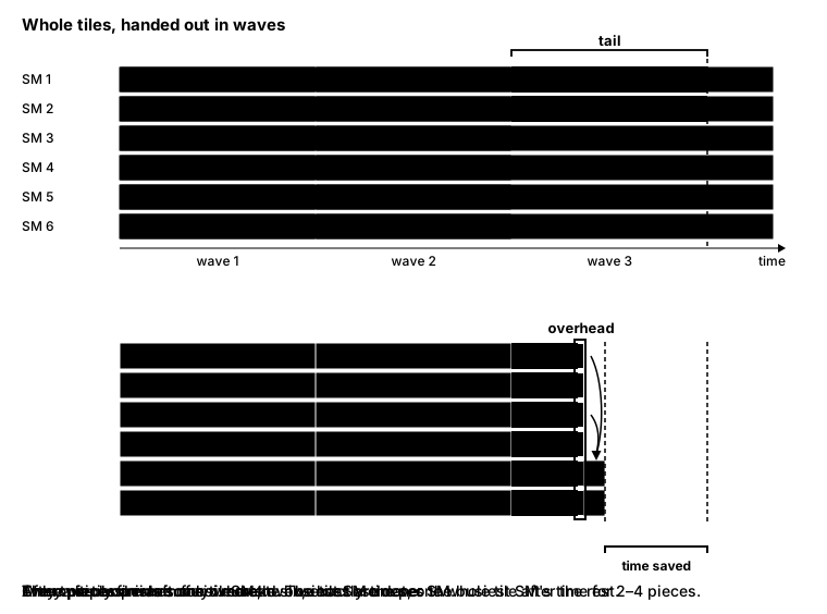
Tile selection still leaves cases where some SMs finish while others have whole tiles left to compute. Stream-K addresses this imbalance by splitting those tiles along and distributing their work across all 48 SMs. The SM computing a tile’s final piece combines the partial sums and writes the result to . Unlike the split-K variant above, this approach leaves the tiles assigned to full waves intact and splits only the work that would form the incomplete wave.
This version improves throughput over the 128×256 kernel by about 11% at and 4% at , although the latter gain is close to the timing variation. The diagram illustrates how splitting the remaining tiles can spread their work more evenly, using six SMs in place of 48:
Reaching that version took two unsuccessful attempts. The first assigned each SM a long sequence of steps that could cross tile boundaries. Although this kept the SMs occupied, they progressed far enough apart to lose L2 reuse, increasing time per tile by about 40%. The second allowed a tile to be divided into as many as 16 pieces and reached only 43% of cuBLAS’s throughput at . Keeping every SM busy was not sufficient when the scheduling also increased the cost of processing a tile.
Restricting each tile to two through four pieces gave better results. As with tile selection, the CPU estimates the work assigned to the busiest SM before launching the kernel. Here the estimate includes an allowance for combining partial sums, so the selection accounts for some of the extra work introduced by splitting. The CPU chooses the candidate with the lowest estimated cost.
Power Throttling
The timing variation became important as the kernels approached cuBLAS’s throughput. A simple multiply-add loop could sustain 2.4 GHz on the GB10, but SGEMM did not hold that clock. Alongside arithmetic, SGEMM moves data through shared memory and registers, drawing enough power to reach this device’s budget. The chip then lowers its clock, a constraint we had not investigated on the T4.
During a 50-second SGEMM run, the driver reported about 95 W with the power limit active throughout, while the clock fell from 2.2 GHz to 2.1 GHz. At 2.1 GHz, the theoretical FP32 peak is about 25.8 TFLOP/s, making cuBLAS’s 17,119 GFLOP/s at roughly two-thirds of that peak.
Horace He’s H100 experiment offers a useful way to explore the effect of power: multiply zero-filled matrices instead of random ones. With fewer bits changing, power draw can fall and the clock can stay higher. Repeating that experiment on the GB10 made these kernels about 10% faster with all-zero inputs. The instructions had not changed, but their input values affected the measured throughput, making the data itself part of the benchmark conditions.
This variation limits what I can conclude from the small lead over cuBLAS. The same kernel’s timing changes by up to 5% between sets of runs. Retiming each size twice in the same session reproduced the 128×256 kernel’s 3–4% lead, but a repeatable lead within those comparisons does not remove the larger variation between sets. For that reason, I describe the result as parity rather than a clear performance advantage.
Profiling Against cuBLAS
The profiler provides another comparison because its runs are brief enough for the kernels to remain at full clock speed. Under those conditions, the 128×256 kernel was again about 4% ahead of cuBLAS, with math-unit utilization at 70% against cuBLAS’s 62%. This supports the throughput comparison under a different run duration, while leaving the longer-run power constraint relevant.
Profiling also exposed a difference I could not explain. Although cuBLAS is closed-source, its counters showed roughly three shared-memory passes for loads that required four in our kernel. I suspected the thread mapping might account for the difference: each half-warp covers two rows of eight outputs, and I estimated that changing the arrangement to a 4×4 square could reduce the pass count to three.
The modified kernel instead required about five passes, with no change in performance. That contradicted the estimate, so I cannot yet explain cuBLAS’s lower count or conclude that matching it would improve throughput under the power limit.
Looking Back
Increasing the outputs per thread eventually brought the kernel to cuBLAS’s throughput, extending the register-tiling idea from Part 1. The smaller patch benefited from a second resident block, while the larger patch provided enough independent work to perform well with one. The useful balance between reuse and concurrency changed as the patch grew, while tile selection and splitting addressed the separate problem of distributing work across the GPU.
I have stopped here for true 32-bit SGEMM. The final 128×256 kernel retained a 3–4% lead over cuBLAS in repeated timings and the profiler comparison, but power-related variation was larger than that margin. I therefore treat the result as approximate parity. Allowing lower-precision inputs would open a different route to much larger gains through tensor cores.
At 2.4 GHz, 48 SMs × 128 cores × 2 flops per cycle gives a theoretical peak of about 29.5 TFLOP/s. A simple multiply-add loop reached 28.9 TFLOP/s, while a read-only kernel measured about 240 GB/s against the specified 273 GB/s bandwidth. ↩︎
Each reported timing is the median of three sets of seven timed runs, collected in one session on an otherwise idle machine. Even within that session, timings for the same kernel varied by up to about 5% as the chip reached its power limit. ↩︎
The double-buffered kernel reached 11,119 GFLOP/s at , compared with cuBLAS’s 10,851. At , the figures were 12,825 and 12,578 respectively; cuBLAS reached 15,575 at . Both implementations used the same layout, with each row padded to a multiple of four floats so the wide loads remained valid at odd sizes. ↩︎