Optimizing Matrix Multiply on CUDA
Why Matrix Multiplication Matters
Most of the time a neural network spends on a GPU goes to one operation, multiplying two matrices. Attention, fully connected layers, and convolutions all reduce to it. The routine that does it for 32-bit floats is called SGEMM (single-precision general matrix multiply), and GPU vendors invest heavily in tuning it. NVIDIA’s version lives in cuBLAS.
For a graduate course at UCSD, my teammate Jerry Ma and I were asked to write our own SGEMM kernel, a function that runs on the GPU, in CUDA for an NVIDIA T4 and get as close to cuBLAS as we could. Our starting point was a correct but naive kernel running at around 100 GFLOP/s (billion floating-point operations per second). Our final kernel reached 4,780 GFLOP/s at , roughly on par with cuBLAS at that size in our measurements. The code is on GitHub.
Much of what we did follows Simon Boehm’s worklog, How to Optimize a CUDA Matmul Kernel for cuBLAS-like Performance, which I’d recommend to anyone curious. This post walks through the same ideas with more background, explaining what each optimization does, why it helps, what we measured on our hardware, and where the remaining performance goes. In late summer of 2026, I returned to this project and built the follow-ups we’d listed on a newer personal GPU, and the post ends with that work.
Counting the Work
To multiply an matrix by an matrix , each output entry is the dot product of row of and column of : multiplications and additions. With outputs, the whole job is floating-point operations. For that’s about 17 billion.
Each output takes multiply-adds, and neighboring outputs read the same data again:
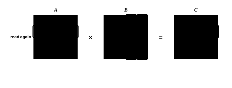
Re-reading the same rows and columns is what every optimization in this post targets, because a T4 can do arithmetic far faster than it can fetch numbers from its main memory:
- Compute: 40 streaming multiprocessors (SMs) × 64 floating-point units × ~1.5 GHz × 2 operations per fused multiply-add ≈ 7,680 GFLOP/s.
- Memory: about 320 GB/s from its off-chip GDDR6 memory, which we’ll call global memory.
Divide one by the other and you get about 24 flops per byte: to keep the arithmetic units busy, a kernel must do at least that much arithmetic for each byte it fetches from global memory. A kernel’s flops per byte fetched is its arithmetic intensity, and each stage below is an attempt to raise it. A naive dot product reads two 4-byte floats for each multiply-add (counts as 2 operations). That gives an arithmetic intensity of 0.25, about 100× short of 24.
Matrix multiply has plenty of reuse to exploit, because every element of is needed by different outputs, and so is every element of . If a kernel fetched each element from global memory only once, its intensity would be , or 512 at , far above 24. Real kernels land in between, and the stages below are steps toward that ceiling.
Running Code on a GPU
Every kernel in this post is written in CUDA, NVIDIA’s extension of C++ for programming its GPUs, and runs on NVIDIA hardware. Other accelerators have their own languages and hardware. Many AMD GPUs, for example, run threads in groups of 64 instead of 32, and Google’s TPUs multiply matrices in large dedicated units rather than across thousands of threads. The terms below are CUDA’s.
The rest of this post relies on three ideas about how a GPU runs code.
Threads come in groups. A CUDA kernel launches thousands of threads. The hardware runs them in groups of 32 called warps, and a warp executes one instruction at a time for all 32 threads in lockstep. Warps are grouped into thread blocks (blocks for short), and each block is assigned to one SM.
Memory is a hierarchy. From slowest and largest to fastest and smallest:
- Global memory (16 GB on the T4) is the off-chip memory from earlier, shared by every thread.
- Shared memory (up to 64 KB per SM) is on-chip, and shared by the threads of one block. It’s something like a scratchpad the programmer manages by hand.
- Registers (64K 32-bit registers per SM) are private to each thread and are the only place arithmetic happens.
Latency is hidden by switching, not waiting. When a warp waits on memory, the SM switches to another warp that’s ready to run. The fraction of an SM’s warp slots that are filled is called occupancy. More warps give the SM more options while it waits, but as we’ll see when we measure our kernel’s occupancy, they aren’t the only way to hide latency.
Optimizing the Kernel
Our kernel went through the stages below, each building on the one before.1
| Stage | Idea | Throughput |
|---|---|---|
| Naive | One thread per output, everything from global memory | ~35–120 |
| Coalesced | Neighboring threads read neighboring addresses | ~550–860 |
| Shared-memory tiling | A block stages tiles of and on-chip | ~650–1,030 |
| 2-D block tiling | Each thread computes an 8×8 patch from registers | up to 4,780 |
| cuBLAS | NVIDIA’s library, for reference | ~2,450–4,570 |
Stage 1: Coalescing
A naive kernel assigns one thread to each output and loops over , the index along the shared dimension (the columns of and the rows of ). Its biggest problem is the way the warp’s 32 threads access memory.
Global memory is read in chunks called transactions. When the 32 threads in a warp ask for 32 consecutive floats, the hardware can combine (coalesce) the requests into a few wide transactions. When they ask for addresses spread far apart, each request becomes its own transaction, and most of every chunk fetched is thrown away.
A comparison of strided and coalesced access for one warp is shown below:
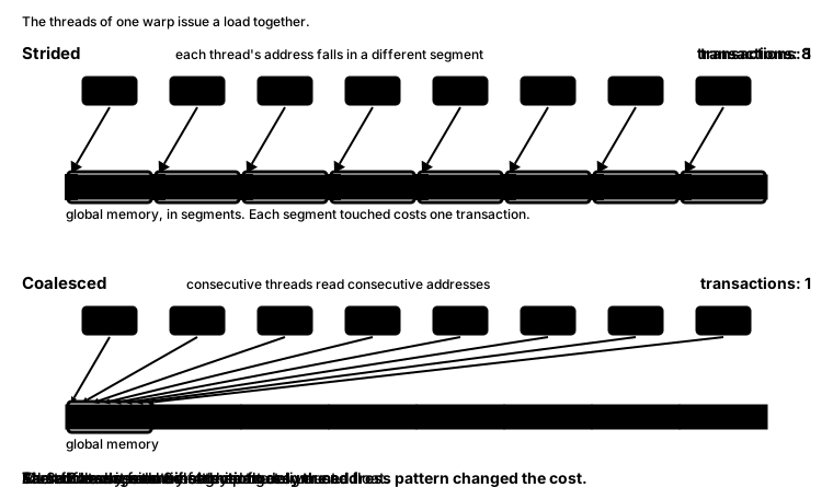
Which pattern you get depends only on how a thread’s ID maps to a row and column of . If consecutive threads in a warp handle consecutive rows, their reads of land floats apart. If they handle consecutive columns, their reads of and writes to are contiguous. The arithmetic is identical either way, yet the coalesced kernel runs roughly an order of magnitude faster than the naive one, because each warp’s loads now combine into a few wide transactions instead of one per thread.
Stage 2: Shared-Memory Tiling
Even coalesced, every thread still streams a whole row of and a whole column of from global memory, and neighboring threads fetch the same values over and over. Shared memory lets a thread block fetch each value once for all of its threads.
The block is responsible for a square tile of . It walks along the shared dimension one slice at a time. For each slice, the threads cooperatively load a tile of and a tile of into shared memory, wait for each other (__syncthreads()), and then every thread computes its partial sums from the on-chip copies.
Each tile is loaded into shared memory once and then read by every thread in the block:
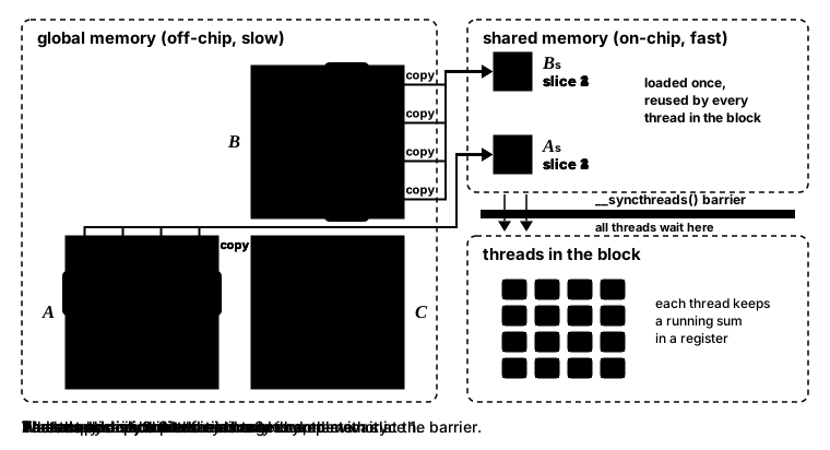
With a T×T tile, each value loaded from global memory is used T times. Arithmetic intensity, which counts only global-memory traffic, rises to about T/4 flops per byte. For a 32×32 tile that’s 8, a 32× improvement over naive on paper. In practice it beat the coalesced kernel by anywhere from about 20% to 70% depending on the size, topping out near 1,000 GFLOP/s.
The speedup fell short of 32× because we moved the bottleneck rather than removing it. Global traffic dropped 32×, but shared-memory traffic didn’t: each multiply-add still reads two operands, now from shared memory instead of global. Those loads don’t count toward arithmetic intensity, but they still cost instructions and shared-memory bandwidth. The threads end up spending most of their time loading operands rather than computing.
Stage 3: Register Tiling
The next step comes in two parts, and both give each thread more work, letting each value it loads feed more than one calculation.
First, 1-D tiling: each thread computes a short column of outputs instead of one. A value it loads from ’s tile can then be reused for every output in that column. According to our report, this nearly doubled throughput.
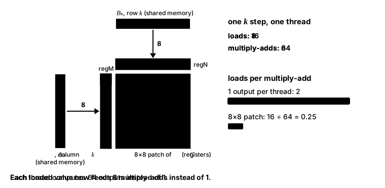
Then, 2-D tiling, where each thread computes an 8×8 patch of . At each step , the thread loads 8 values from a column of ’s tile and 8 values from a row of ’s tile into registers, then multiplies every value by every value. This is an outer product, and it gets 64 multiply-adds from 16 loads.
The per-thread outer product is shown below:
The inner loop of our final kernel looks like this (unrolling pragmas omitted):
for (uint dotIdx = 0; dotIdx < TILEDIM_K; ++dotIdx) {
    for (uint i = 0; i < TILESCALE_M; ++i)
        regM[i] = As[threadRow * TILESCALE_M + i][dotIdx];
    for (uint i = 0; i < TILESCALE_N; ++i)
        regN[i] = Bs[dotIdx][threadCol * TILESCALE_N + i];
    for (uint m = 0; m < TILESCALE_M; ++m)
        for (uint n = 0; n < TILESCALE_N; ++n)
            threadResults[m][n] += regM[m] * regN[n];
}
Our final configuration:
- Block: 16×16 = 256 threads.
- Block tile: 128×128 outputs of (16 threads × 8 outputs each way).
- slice: 32, meaning each slice stages a 128×32 tile of and a 32×128 tile of , 32 KB in total.
- Per thread: an 8×8 patch, which is 64 accumulators plus 16 operand registers.
This configuration is essentially kernel 5 in Boehm’s worklog. It took us from ~1,000 to 4,780 GFLOP/s.
Getting here was the hardest part of the project, even though the code is short. We first misread what a “block tile” was, and built a version where each thread tried to compute a large tile on its own. It was slower than 1-D tiling, because loads to shared memory stopped coalescing, and each thread carried more work than it could keep in registers. A conversation with our TA made us realize that a block tile is the output of the whole thread block, which is then divided among the threads. The rest of the kernel follows the same pattern, with the block tile sized for shared memory and each thread’s patch sized for its registers.
Tuning the Shape
Because the block and per-thread sizes interact, we swept a few combinations:
| Threads per block | Outputs per thread | Block tile | Throughput |
|---|---|---|---|
| 32×32 | 2×2 | 64×64 | ~2,210 |
| 8×8 | 8×8 | 64×64 | ~2,470 |
| 16×16 | 4×4 | 64×64 | ~3,720 |
| 16×16 | 8×8 | 128×128 | 4,780 |
More outputs per thread help, as long as the registers can hold them. At 2×2 outputs per thread, loads dominate. With 16×16 threads, going from 4×4 to 8×8 outputs per thread (a 128×128 block tile) reuses each loaded value enough to keep the arithmetic units busy.
The largest configuration didn’t win at every size. At , the 128×128 configuration was the slowest of the four, at under 500 GFLOP/s. And every configuration lost throughput when was just past a multiple of the tile size, which we’ll call an odd size:
| 512 | 1023 | 1024 | 1025 | 2048 | 2049 | |
|---|---|---|---|---|---|---|
| Throughput | 2,167 | 3,830 | 3,920 | ~2,900 | 4,780 | 4,181 |
When isn’t a multiple of 128, the tiles at the right and bottom edges hang off the matrix. Every load and store needs a bounds check, and out-of-range lanes fill in zeros, sending threads in the same warp down different branches. That divergence costs something, but it can’t explain why is so much slower than , since both need the same checks. Wave quantization, explained after we measure the kernel’s occupancy later in the post, accounts for both results.
Performance Analysis
The roofline
A roofline plot (Williams, Waterman, and Patterson) puts arithmetic intensity on the x-axis and throughput on the y-axis. The “roof” has two parts. On the left, a slope: with little reuse, throughput is capped by memory bandwidth times intensity. On the right, a flat ceiling: past the ridge point (about 24 flops per byte on the T4), the cap is peak compute.
The 32×32 shared-memory kernel and our final 128×128 kernel sit on the roofline as shown below:
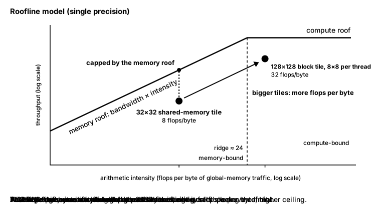
With 128×128 tiles, the kernel does about 32 flops per byte it reads from global memory. That puts it past the ridge, where memory bandwidth no longer limits it. Its 4,780 GFLOP/s is 62% of peak compute. The missing 38% goes to the SM’s other work, such as shared-memory loads, index math, and barriers, not to waiting on global memory.2
Occupancy
Two resources decide our kernel’s occupancy, the filled share of an SM’s 32 warp slots.
Registers. A hand count suggests about 80 registers per thread: 64 accumulators plus 16 operands. The real count is higher, because the compiler also keeps indices, pointers, and loop counters in registers. ptxas -v reports 172 per thread when targeting the T4.3 A block of 256 threads at 172 registers each needs about 44,000 registers. Out of the SM’s 65,536, that leaves room for only one block.
Shared memory. Each block stages 32 KB of tiles. With 64 KB per SM on the T4, shared memory alone would allow two blocks. Registers are the tighter limit.
One block of 256 threads is 8 warps, which fill 8 of the SM’s 32 warp slots: 25% occupancy. Even with three-quarters of the SM’s warp slots empty, the kernel reached 62% of peak. Vasily Volkov’s talk Better Performance at Lower Occupancy explains why: an SM can hide latency with many warps, or with fewer warps that each have lots of independent work. With 64 independent accumulators per thread, the SM still has dozens of multiply-adds it can issue while one load is in flight.
Why small and odd-sized matrices were slow
One block per SM also explains two slowdowns we measured earlier: small matrices run slowly, and a size just past a multiple of 128 runs slower than the size just below it. The GPU runs blocks in waves: each wave fills every SM with as many blocks as fit on it at once. Speed at a given size follows from three facts:
- Each block computes one 128×128 tile of , and an matrix needs blocks.
- With one block per SM, a wave holds 40 blocks.
- A partial wave takes as long as a full one.
Small matrices produce fewer blocks than there are SMs:
- produces only 4 blocks, leaving 36 of the 40 SMs idle.
- gives 16 blocks, leaving 24 of the 40 SMs idle.
Just past a multiple of 128, one extra row and column of tiles can add a whole wave:
- and both give 8×8 = 64 blocks: a full wave of 40, then a partial wave of 24. Both sizes take two waves and run at nearly the same speed.
- needs 9×9 = 81 blocks: two full waves, then a third wave with a single block. Taking three waves instead of two, should run at about two-thirds of ’s speed. That predicts roughly 2,600 GFLOP/s, and we measured about 2,900.
- gives 17×17 = 289 blocks, which takes eight waves instead of ’s seven. It should run at 7/8 of ’s 4,780 GFLOP/s. That predicts about 4,180, and we measured 4,181.
This effect is called wave quantization (or the tail effect), and it’s why cuBLAS picks different kernels for different sizes. It explains the odd-size drops, and also why smaller tiles won at : a 64×64 tile turns that matrix into 16 blocks instead of 4, giving more SMs work.
What We’d Do Next
Our final kernel stops at Boehm’s kernel 5. The remaining steps in his worklog each address a limit we found above:
- Fit two blocks per SM. Shared memory already has room for two, but registers don’t. Capping them at 128 per thread with
__launch_bounds__(256, 2)should fit a second block, at the cost of some spilling.4 Two blocks per SM would also halve the number of waves, softening the wave quantization problem. - Fix shared-memory bank conflicts. Shared memory is split into 32 banks, and threads in a warp that hit the same bank at once take turns, one pass each. Our reads from ’s tile likely put about 2 threads on each bank, so each read takes about 2 passes instead of 1. Padding the arrays, or changing which columns each thread reads, are the usual fixes.
- Vectorized loads. Loading four floats per instruction (
float4) instead of one means 4× fewer load instructions. - Warp tiling. Give each warp a compact rectangle of the block tile instead of full-width rows. Each warp then reads fewer values from shared memory per step.
- Double buffering. Loading the next slice while computing the current one hides the
__syncthreads()wait.
Round Two on a GB10
Almost two years later, I implemented that list. Since the T4 was a course machine I no longer have, these measurements come from an NVIDIA GB10, the Blackwell chip in NVIDIA’s DGX Spark desktop.
The GB10 differs from the T4 in several ways:
- It has 48 SMs instead of 40.
- Each SM has 100 KB of shared memory instead of 64 KB, and the same 64K registers.
- It does almost 4× more arithmetic per second: about 29.6 TFLOP/s against the T4’s 7.68.5
- Its memory is shared with the CPU and has about 15% less bandwidth than the T4’s: 273 GB/s against 320.6
None of the numbers below can be compared with the T4 numbers earlier in the post. Instead, every step is compared with cuBLAS on the same GPU, with TF32 disabled so both do true 32-bit math.
Each step is a separate kernel, built on top of the one before, in a small standalone benchmark (next/ in the repo). Every result is checked against cuBLAS.7
| Step | vs cuBLAS | vs cuBLAS | ||
|---|---|---|---|---|
| Our course kernel | 9,661 | 60% | 10,723 | 63% |
| + two blocks per SM | 11,508 | 71% | 12,616 | 74% |
+ float4 loads, transposed | 13,882 | 86% | 14,181 | 83% |
| + bank-conflict fix | 14,323 | 88% | 14,623 | 85% |
| + warp tiling | 14,234 | 88% | 14,812 | 87% |
| + warp tiling, | 14,687 | 91% | 15,209 | 89% |
| + double buffering () | 14,933 | 92% | 15,392 | 90% |
| cuBLAS | 16,204 | 100% | 17,119 | 100% |
Step by step, with gains at :
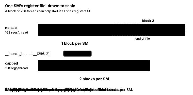
Two blocks per SM: +19%. On this GPU the compiler gives our kernel 168 registers per thread, again enough for only one block per SM. __launch_bounds__(256, 2) tells the compiler two things: each block has at most 256 threads, and at least two blocks should fit on an SM at once. Two blocks of 256 threads split the SM’s 65,536 registers into 128 per thread.
By spilling 72 bytes per thread, or 18 floats, the compiler fits the kernel into that budget, and two blocks now run on each SM, as we predicted after the T4 runs. The second block hides more latency than the extra loads and stores of those spills add. The cap has two other costs: the compiler has fewer spare registers for starting loads early, and blocks of more than 256 threads can no longer launch. The cap decides whether a second block fits in the SM’s register file:
float4 loads with transposed: +21%. Each load instruction from global memory now fetches four floats instead of one, so a thread issues 4× fewer of them. All of this step’s gain comes from those wider loads.
Following Boehm, this step also stores ’s tile transposed in shared memory, with its rows turned into columns. The 8 values of a thread needs at each step used to sit in one column, 32 floats apart, but now they sit side by side in one row. I expected that to let a thread read them with 2 wide reads instead of 8 narrow ones. For one row of ’s tile, the loads and the transposed layout look like this:
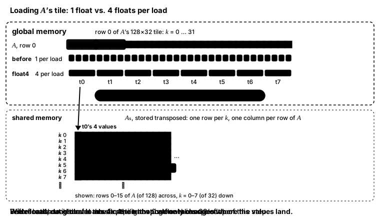
In the original layout, one row’s values for steps through already sit side by side, and the compiler was already reading them with one wide read. The transpose saved no reads: both versions issue the same number of shared-memory reads.8
The transpose stays because a later kernel with a bigger tile needs it: without the transpose, that kernel ran 2–4% slower. In the 128×128 kernels of round two, the transposed writes into shared memory cause bank conflicts, which a later step reduces.
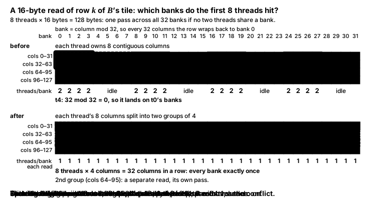
Bank-conflict fix: +3%. Shared memory’s 32 banks each hold every 32nd float: columns 0 and 32 of ’s tile sit in the same bank. As we saw earlier, threads in a warp that read the same bank at once take turns, one pass each.
Before the fix, each thread read 8 neighboring columns of from shared memory, 4 at a time: thread 0 read columns 0–7, thread 1 read 8–15, and so on. Thread 4’s first read, columns 32–35, then hit the same banks as thread 0’s columns 0–3, and the two took turns.
The fix splits each thread’s 8 columns into two groups of 4, placed 64 columns apart. Thread 0 reads columns 0–3 and 64–67, and thread 1 reads 4–7 and 68–71. Eight threads reading their first group now cover columns 0–31, so each bank serves exactly one thread.9 The second group starts at column 64 because the 16 threads across the tile fill columns 0–63 with their first groups. Column 64 maps to the same bank as column 0, but the second group is a separate read and never competes with the first. The same split applies to rows of : each thread’s 8 rows also become two groups of 4, 64 rows apart. Here’s how the two layouts map onto the banks:
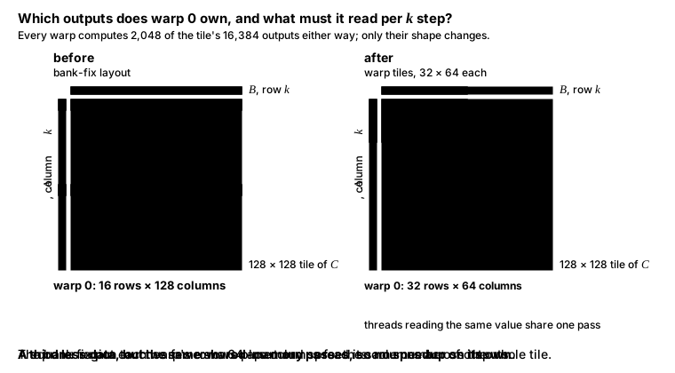
Warp tiling: no gain on its own. Before, each warp owned 16 rows of the block tile, each 128 outputs wide. Now it owns a 32×64 region. At each step it reads 32 values of plus 64 of , 96 in all, instead of 16 plus 128, or 144. The speed didn’t change: the reads it removed were already cheap. Threads in a warp that read the same value get it in a single pass, so most of those 144 values cost nothing extra. The profiler counted the same number of shared-memory passes, about 50 million, before and after.10 Warp tiling changes which outputs one warp owns:
Smaller slice: +3%. Shrinking the slice from 32 to 16 values deep helped by 3%. A possible reason shows up in the profiler. Storing ’s tile transposed causes heavy bank conflicts on the writes, and the smaller slice cuts those conflicts by more than half.11 The 128×128 fallback tile for odd sizes, described later, avoids them by keeping untransposed.12
Double buffering: +2%. Loading the next slice while computing the current one helped less than I expected. The likely reason is that with two blocks per SM, one block’s loads already overlap the other block’s math. The figure shows how the second buffer hides loads, and why a second block had already hidden most of them:
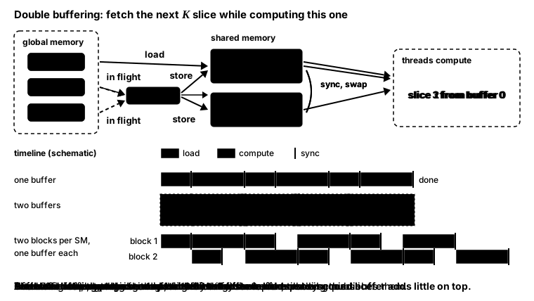
Together, the steps took the kernel from about 60% of cuBLAS to about 90%.
At odd sizes such as and , the final kernel ran about 2% faster than cuBLAS. cuBLAS slows down at odd sizes too: going from to costs it about 30% of its speed.1314
I expected two blocks per SM to help odd sizes the most, since it halves the number of waves, but at it gained nothing. At 81 blocks for 48 SMs, some SMs must run two blocks either way. With one block per SM, they run the two one after the other. With two per SM, they run both at once, each at about half speed, and finish no sooner.
After round two, our kernel was still about 10% slower than cuBLAS at large sizes.
Closing the Gap to cuBLAS
I expected asynchronous copies, a hardware feature the GB10 has and the T4 lacks, to close that 10% gap, but they didn’t. What closed it was giving each thread a bigger share of the output, the register-tiling idea from the T4 taken one step further.15
| Step | vs cuBLAS | vs cuBLAS | ||
|---|---|---|---|---|
| Double buffering (from round two) | 14,933 | 92% | 15,392 | 90% |
| + asynchronous copies | 14,490 | 89% | 15,384 | 90% |
| + 16×8 outputs per thread, 128×256 tile | 16,625 | 103% | 17,839 | 104% |
| cuBLAS | 16,204 | 100% | 17,119 | 100% |
Asynchronous copies: no gain. NVIDIA added the cp.async instruction in its Ampere generation, which came after the T4’s Turing and before the GB10’s Blackwell. It copies data from global to shared memory without passing it through registers, which lets a block queue up slices ahead of time. Each queued slice gets its own buffer, called a stage. With two stages, each holding a slice of depth 16, the cp.async kernel ran at the same speed as plain double buffering. With four stages of depth 8, which take the same total shared memory as two of depth 16, it ran about 5% slower.
Small probe kernels showed that loading did cost time: a variant of the kernel with the global loads removed ran almost 30% faster. But a variant that re-read the same slice every step, never waiting on global memory, ran exactly as fast as the real kernel.16 So the time went to the instructions that move each tile, loading it from global memory and storing it into shared memory, not to waiting on memory. cp.async removes few of those instructions, because ’s tile is stored transposed and has to be copied one 4-byte float per instruction.
A bigger share per thread: the gap closes. According to cuBLAS’s own logs, at it runs a CUTLASS kernel whose threads each compute 128 outputs, twice our 64. So I grew each thread’s patch of from 8×8 to 16×8. With the block still at 256 threads, its tile grows from 128×128 to 128×256. It still loads with cp.async, in two stages.
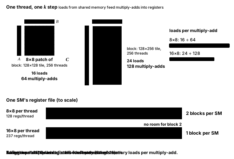
A bigger patch reuses each loaded value more. At each step, a thread now loads 24 values from shared memory to do 128 multiply-adds, instead of 16 for 64. Each value of still feeds 8 multiply-adds, but each value of now feeds 16 instead of 8. In the profiler, the math units were busy 70% of the time instead of 58%.
The bigger patch costs registers: holding 128 running sums takes 237 registers per thread, which puts the kernel back at one block per SM, undoing the first step of round two. As on the T4, one block per SM didn’t hurt, because each thread now updates 128 independent sums instead of 64.
The 128×256 kernel closed the gap: at both and it runs 3–4% faster than cuBLAS, a margin within the run-to-run spread. For one thread, the cost per step changes as follows:
Odd sizes: picking a tile per size. A 128×256 tile fits some sizes badly. At , the last column of tiles covers a single column of , and at there are only 32 tiles for 48 SMs. So the final kernel chooses between three versions for each size:
- the big 128×256 tile
- a 128×128 tile, whose 128 threads each still compute 16×8 outputs
- a split-K version, which splits the dimension three ways so more SMs have work when there are few tiles.
For each size, the host picks the version that leaves the busiest SM the least work. With that choice, the kernel ran at 115% of cuBLAS at and 114% at . At it matched cuBLAS, up from 86% with the 128×256 tile alone.12
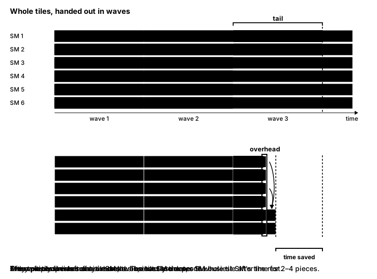
Splitting the last wave: stream-K. One last change helped at sizes whose final wave of tiles only partly fills the GPU. Instead of letting most SMs sit idle during that wave, the kernel splits its tiles along and spreads the pieces across all 48 SMs, a scheme called stream-K. Unlike the split-K version above, which splits every tile, stream-K splits only the tiles in the last wave. The SM that finishes a tile’s last piece adds up the other pieces’ sums and writes .
At this was about 11% faster than the 128×256 tile alone. At it was about 4% faster, close to the run-to-run spread.17 Splitting changes how the last wave is spread across the SMs:
The chip hits its power limit. A plain multiply-add loop held the full 2.4 GHz clock, but SGEMM draws more power, and the driver reported the chip at its power limit for a whole run.18 The clock slid from 2.2 to 2.1 GHz as the chip warmed up. At 2.1 GHz the peak is about 25.8 TFLOP/s, and cuBLAS reaches about two-thirds of that.
The same kernels also ran about 10% faster on matrices of zeros, which take less energy to multiply. So on this chip, energy per flop matters as much as instruction count, and results drift by a few percent with how warm the chip is.
The profiler’s runs are short enough that the chip never reaches the cap. In those runs, the big-tile kernel was about 4% faster than cuBLAS’s kernel. It also kept the math units busier, 70% of the time against 62%.
For the same number of shared-memory loads, cuBLAS’s kernel makes about 3 bank passes for every 4 of ours, because of how it assigns threads to outputs in its tile. When I copied that assignment, my kernel went to about 5 passes for every 4 it made before, and the speed didn’t change. How cuBLAS gets its savings, and whether they matter under the power cap, is still an open question for me.
Tensor cores would be much faster still, but by rounding the inputs to lower precision they solve a different problem.
Looking Back
Before this project, I thought of GPU performance as a matter of parallelism: more threads, more speed. The biggest lesson was that parallelism is the easy part, since the naive kernel already had one thread per output. Every real gain came from data movement, from getting a warp’s accesses to line up, a block to share what it loaded, and a thread to reuse what it held. The arithmetic barely changed from the first kernel to the last.
The second lesson was to check every explanation against the hardware’s hard limits. Numbers like registers per thread, shared memory per SM, and the count of SMs explained our results better than any intuition about “memory-bound” or “compute-bound”. The compiler’s register report and a bit of arithmetic about waves accounted for results that guessing hadn’t.
Because the repository only keeps the naive and final versions as code, for the middle stages I describe the idea and quote approximate numbers from our report. ↩︎
Intensity here is measured per byte, not per element loaded, since the ridge point is defined in bytes. The figure of 32 flops per byte assumes each value is read from global memory once per tile, and ignores caches. ↩︎
The exact count varies slightly between CUDA versions. A second block would only fit at or below 128 registers per thread. ↩︎
A thread spills when it needs more values at once than its registers can hold. The compiler moves the extras to local memory, which is private to each thread but lives in the GPU’s slow main memory. Each spilled value costs an extra store and a later load. ↩︎
The peak comes from 48 SMs × 128 cores × 2 flops per cycle at its 2.4 GHz clock. A plain multiply-add loop reached 28.9 TFLOP/s. ↩︎
A simple read kernel reached about 240 GB/s. ↩︎
Each figure is the median of 3 sets of 7 timed runs, all measured in one session on an otherwise idle machine. Sets of the same kernel differed by up to about 5%, because the chip hits its power limit, as described below. ↩︎
In the compiled code, each thread issues 128 wide shared-memory reads per slice in both versions. At , the profiler counted 16.8 million shared-memory read instructions for each. ↩︎
In the profiler, the bank-conflict counter for shared-memory reads fell from 33.6 million to 54 thousand, and the average number of passes per read fell from 5 to 3. That average covers every shared-memory read in the kernel, not just these reads of , so it doesn’t fall to 1. ↩︎
Traffic to global memory didn’t change either: each block still computes a 128×128 tile of from the same slices of and , leaving the arithmetic intensity measured against global memory unchanged. The kernel wasn’t compute-bound: even after the last step of round two, the math units were busy only 58% of the time. ↩︎
The transposed stores cost about 6 extra passes per store at a slice of 32. ↩︎
The 128×128 version stores ’s tile untransposed, so it can copy 16 bytes at a time instead of 4. That avoids the bank conflicts on transposed stores from round two. A 256×128 tile, with twice as many rows of to copy, was 6–10% slower than 128×256. ↩︎ ↩︎
At the final kernel ran at 11,119 GFLOP/s against cuBLAS’s 10,851, and at at 12,825 against 12,578. cuBLAS ran at 15,575 at . ↩︎
To make the wide loads legal at odd sizes, the benchmark pads each row to a multiple of 4 floats, and cuBLAS got the same padded layout. ↩︎
The explanations below come from small probe kernels, instruction counts in the compiled code, cuBLAS’s own logs, and the profiler. ↩︎
At the double-buffered kernel ran at about 15.7 TFLOP/s, and the variant that re-read one slice ran at the same speed. With its global loads removed it reached 20.2, and adding back only the stores into shared memory brought it to 18.7. The profiler agreed: warps waiting on global memory made up only 5% of its stall samples, while waiting on shared memory and at barriers made up 18%. Its transposed stores into shared memory still took about 4 passes each because of bank conflicts. ↩︎
Two earlier versions of this split failed. Giving each SM one contiguous range of let the SMs drift apart until they stopped sharing data in L2, and each tile ran about 40% slower. Allowing up to 16 pieces per tile made the odd sizes far worse, dropping to 43% of cuBLAS. The version that worked uses 2 to 4 pieces per tile, and the host picks the split that leaves the busiest SM the least work. In the code, the split tiles actually run first and the whole tiles after them. The total work is the same, but it means the last wave in the stream-K figure is really the first. ↩︎
The multiply-add loop reached 98% of the chip’s peak. During a 50-second SGEMM run, the chip drew about 95 W. ↩︎